Updated on 2019-05-29 with clarifications on Istio’s mixer configuration for the “tuned” benchmark, and adding a note regarding performance testing with the “stock” configuration we used.

The Istio community has updated the description of the “evaluation configuration” based on the findings of this blog post. While we will not remove the original data from this blog post for transparency reasons, we will focus on data of the “tuned istio” benchmark for comparisons to linkerd.

Motivation

Over the past few years, the service mesh has rapidly risen to prominence in the Kubernetes ecosystem. While the value of the service mesh may be compelling, one of the fundamental questions any would-be adopter must ask is: what’s the cost?

Cost comes in many forms, not the least of which is the human cost of learning any new technology. In this report we restrict ourselves to something easier to quantify: the resource cost and performance impact of the service mesh at scale. To measure this, we ran our service mesh candidates through a series of intensive benchmarks. We consider Istio, a popular service mesh from Google and IBM, and Linkerd, a Cloud Native Computing Foundation (CNCF) project.

Buoyant, the original creators of Linkerd, approached us to perform this benchmark and tasked us with creating an objective comparison of Istio and Linkerd. As this allowed us to dive more deeply into these service mesh technologies, we kindly accepted the challenge.

It should be noted that Kinvolk currently has ongoing client work on Istio. Our mission is to improve open source technologies in the cloud native space and that is the spirit by which we present this comparison.

We are releasing the automation for performing the below benchmarks to the Open Source community. Please find our tooling at https://github.com/kinvolk/service-mesh-benchmark .

Goals

We had three goals going into this study:

1. Provide a reproducible benchmark framework that anyone else can download and use.
2. Identify scenarios and metrics that best reflect the operational cost of running a service mesh.
3. Evaluate popular service meshes on these metrics by following industry best practices for benchmarking, including controlling for sources of variability, handling coordinated omission, and more.

Scenario

We aim to understand mesh performance under regular operating conditions of a cluster under load. This means that cluster applications, while being stressed, are still capable of responding within a reasonable time frame. While the system is under (test) load the user experience when accessing web pages served by the cluster should not suffer beyond an acceptable degree. If, on the other hand, latencies would regularly be pushed into the seconds (or minutes) range, then a real-world cluster application would provide a bad user experience, and operators (or auto-scalers) would scale out.

In the tests we ran, the benchmark load - in terms of HTTP requests per second - is set to a level that, while putting both application and service mesh under stress, also allows traffic to still be manageable for the overall system.

Metrics

rps, User Experience, and Coordinated Omission

HTTP traffic at a constant rate of requests per second (rps) is the test stimulus, and we measure response latency to determine the overall performance of a service mesh. The same rps benchmark is also performed against a cluster without any service mesh (“bare”) to understand the performance baseline of the underlying cluster and its applications.

Our benchmarks take Coordinated Omission into account, further contributing towards a UX centric approach with objective latency measurement. Coordinated Omission occurs when a load generator issues new requests only after previously issued requests have completed, instead of issuing a new request at the point in time where it would need to be issued to fulfill the requests per second rate requested from the load generator.

As an example, if we would want to measure latency with a load of 10 requests per second, we’d need to send out a new request every 100 milliseconds, using a constant request rate of 10 Hz. But when a load generator waits for completion of a request that takes longer than 100ms, the rps rate will not be maintained - only 9 (or fewer) requests will be issued during that second instead of the requested 10. High latency is only attributed to a single request even though objectively, successive requests also experience elevated latency - not because these take long to complete, but because they are issued too late. There are two drawbacks with this behaviour: high latency will only be attributed to a single request, even though succeeding requests suffer elevated latency, too (as called out before - not because the results are late, but the requests are issued too late to begin with). And secondly, the application / service mesh under load is granted a small pause from ongoing load during the delayed response, as no new request is issued when it would need to be to match the requested rps. This is far from the reality of a “user stampede” where load quickly piles up in high latency situations.

For our benchmarks, we use wrk2 to generate load and to measure round-trip latency from the request initiator side. wrk2 is a friendly fork, by Gil Tene, of the popular http benchmark tool wrk , by Will Glozer. wrk2 takes requested throughput as parameter, produces constant throughput load, eliminates Coordinated Omission by measuring latency from the point in time where a request should have been issued, and also makes an effort to “catch up” if it detects that it’s late, by temporarily issuing requests twice as fast as the original RPS rate. wrk2 furthermore contains Gil Tene’s “HDR Histogram” work, where samples are recorded without loss of precision. Longer test execution times contribute to higher precision, thus giving us more precise data particularly for the upper percentiles we are most interested in.

For the purpose of this benchmark, we extended the capabilities of wrk2, adding the handling of multiple server addresses and multiple HTTP resource paths. We do not consider our work a fork and will work with upstream to get our changes merged.

Performance

For evaluating performance we look at latency distribution (histograms), specifically at tail latencies in the highest percentiles. This is to reflect this benchmark’s focus on user experience: a typical web page or web service will require more than one, possibly many, requests to perform a single user action. If one request is delayed, the whole action gets delayed. What’s p99 for individual requests thus becomes significantly more common in more complex operations, e.g. a browser accessing all the resources a web page is made of in order to render it - that’s why p99 and higher percentiles matter to us.

Resource Consumption

Nothing comes for free - using a service mesh will have a cluster consume more resources for its operation, taking resources away from business logic. In order to better understand this impact we measure both CPU load of, and memory consumed by the service mesh control plane, and the service mesh’s application proxy sidecars. CPU utilization and memory consumption are measured in short intervals on a per-container level during test runs, the maximum resource consumption of components during individual runs is selected, and the median over all test runs is calculated and presented as a result.

We observed that memory consumption peaks at the end of a benchmark run. This is expected, since (as outlined above) wrk2 issues a constant throughput rate - load will pile up when latency increases over a certain threshold - so memory resources, once allocated, are unlikely to be freed until the benchmark is over. CPU utilization per time slice also stayed at high levels and never broke down during runs.

Benchmark Set-up

The Cluster

We use automated provisioning for our test clusters for swift and easy cluster set-up and teardown, allowing for many test runs with enough statistical spread to produce robust data.

For the benchmarks run during our service mesh performance evaluation, we used a cluster of 5 workers. Each worker node sports a 24 core / 48 thread AMD EPYC(r) CPU at 2.4GHz, and 64 GB of RAM. Our tooling allows for a configurable number of nodes, allowing for re-running these tests using different cluster configurations.

Load is generated and latency is measured from within the cluster, to eliminate noise and data pollution from ingress gateways - we’d like to fully focus on service meshes between applications. We deploy our load generator as a pod in the cluster, and we reserve one cluster node for load generation / round-trip latency measurement, while using the remaining four nodes to run a configurable number of applications. In order to maintain sufficient statistical spread, we randomly pick the “load generator” node for each run.

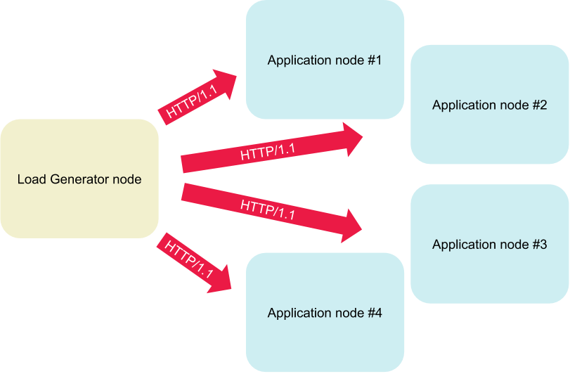
One random node is picked before each run and reserved exclusively for the load generator. The remaining nodes run the application under load.

For the purpose of this test we used Packet as our IaaS provider; the respective server type used for worker nodes is c2.medium. Packet provides “bare metal” IaaS - full access to physical machines - allowing us to eliminate neighbour noise and other contention present in virtualized environments.

Cluster Applications

As discussed in the “Metrics” section above, we use wrk2 to generate load, and augment the tool to allow benchmarks against multiple HTTP endpoints at once.

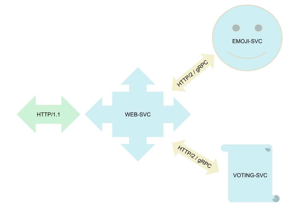
The application we use to run the benchmark against is “Emojivoto”, which comes as a demo app with Linkerd, but is not related to Linkerd functionality, or to service meshes in general (Emojivoto runs fine without a service mesh). Emojivoto uses a HTTP microservice by the name of web-svc (of kind: load-balancer) as its front-end. web-svc communicates via gRPC with the emoji-svc and voting-svc back-ends, which provide emojis and handle votes, respectively. We picked Emojivoto because it is clear and simple in structure, yet contains all elements of a cloud-native application that are important to us for benchmarking service meshes.

The emojivoto application consists of 3 microservices.

However, benchmarking service meshes with only a single application would be a far cry from real-world use cases where service meshes matter - those are complex set-ups with many apps. In order to address this issue yet keep our set-up simple, we deploy the Emojivoto app a configurable number of times and append a sequence counter to service account and deployment names. As a result, we now have a test set-up that runs web-svc-1, emoji-svc-1, voting-svc-1 alongside web-svc-2, emoji-svc-2, voting-svc-2, etc. Our load generator will spread its requests and access all of the apps' URLs, while observing a fixed overall rps rate.

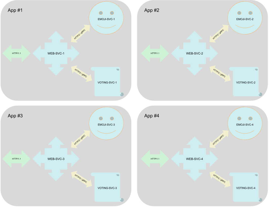
Looping over the deployment yaml and appending counters to app names allows us to deploy a configurable number of applications.

On Running Tests and Statistical Robustness

As we are using the datacenters of a public cloud provider - Packet - to run our benchmarks, we have no control over which specific servers are picked for individual deployments. The age of the machine and its respective components (memory, CPU, etc), its position in the datacenter relative to the other cluster nodes (same rack? same room? same fire zone?), and the state of the physical connections between the nodes all have an impact on the raw data any individual test run would produce. The activity of other servers unrelated to our test, but present in the same datacenter, and sharing the same physical network resources, might have a derogatory effect on test runs, leading to dirty benchmark data. We apply sufficient statistical spread with multiple samples per data point to eliminate volatile effects of outside operations on the same physical network when comparing data points relative to each other - i.e. Istio’s latency and resource usage to Linkerd’s. We furthermore use multiple clusters in different datacenter with implicitly different placement layouts to also help drawing absolute conclusions from our data.

In order to achieve sufficient statistical spread we execute individual benchmark runs twice to derive average and standard deviation. We run tests in two clusters of identical set-up in parallel to make sure our capacity does not include a “lemon” server (degraded hardware) or a bad switch, or has nodes placed at remote corners in the datacenter.

A typical benchmark test run would consist of the following steps. These steps are run on two clusters in parallel, to eliminate the impact of “lemon” servers and bad networking.

=> Before we start, we reboot all our worker nodes.

=> Then, for each of “istio-stock”, “istio-tuned”, “linkerd”, “bare”, do, on 2 clusters simultaneously:

1. Install the service mesh (skip if benchmarking “bare”, i.e. w/o service mesh)
2. Deploy emojivoto applications
3. Deploy benchmark load generator job
4. Wait for the job to finish, while pulling resource usage metrics every 30 secs
5. Pull benchmark job logs which contain latency metrics
6. Delete benchmark load generator job and emojivoto
7. Uninstall service mesh
8. Goto 1. to benchmark the next service mesh (linkerd -> istio -> bare)
9. After all 4 benchmarks concluded, start again with the first service mesh,
   and run the above twice to gain statistical coverage

Reproducibility

We provisioned the clusters using Kinvolk’s recently announced Kubernetes distribution, Lokomotive. The code for automating both the provisioning of the test clusters as well as for running the benchmarks is available under an open source license in the Github repo. This is to allow for reproducing the benchmark results and hopefully accepting improvements from others.

As mentioned above, we are also releasing our extensions to wrk2, available here: https://github.com/kinvolk/wrk2 .

Benchmark runs and observations

We benchmarked “bare” (no service mesh), “Istio-stock” (without tuning), “Istio-tuned”, and “Linkerd” with 500 requests per second, over 30 minutes. Benchmarks were executed twice successively per cluster, in 2 clusters - leading to 4 samples per data point. The test clusters were provisioned in separate data centers in different geographical regions - one in Packet’s Sunnyvale datacenter, and one in the Parsippany datacenter in the New York metropolitan area.

Service mesh versions used

Istio - “stock” and “tuned”

We ran our benchmarks on Istio release 1.1.6 , which was current at the time we ran the benchmarks. We benchmarked both the “stock” version that users would receive when following the evaluation set-up instructions (update: a warning has been added to the evaluation instructions following the initial release of this blog post; see details below) as well as a “tuned” version that removed memory limitations and disabled a number of Istio components, following various tuning recommendations. Specifically, we disabled Mixer’s Policy feature (while leaving telemetry active to retain feature parity with Linkerd), and disabled Tracing, Gateways, and the Prometheus add-on configuration.

Update 2019-05-29 @mandarjog and @howardjohn reached out to us via a github issue filed to the service mesh benchmark project , raising that:

• The “stock” Istio configuration, while suitable for evaluation, is not optimized for performance testing.
  • This led to a change on the Istio project website to call out this limitation explicitly.
• The “tuned” Istio configuration was still enforcing a restrictive CPU limit in one case.
  • We removed the limitation and increased the limits in accordance with suggestions we received in the github issue.
  • We re-ran a number of tests but did not observe significant changes from the results discussed below - the relations of bare, Linkerd, and Istio latency remained the same. Also, Istio continued to expose latencies in the minute range when being overloaded at 600rps. Please find the re-run results in the github issue at https://github.com/kinvolk/service-mesh-benchmark/issues/5#issuecomment-496482381 .

Linkerd

We used Linkerd’s Edge channel, and went with Linkerd2-edge-19.5.2 , which was the latest Linkerd release available at the time we ran the benchmarks. We used linkerd as-is, following the default set-up instructions , and did not perform any tuning.

Gauging the limits of the meshes under test

Before we started our long-running benchmarks at constant throughput and sufficient statistical spread, we gauged throughput and latency of the service meshes under test in much shorter runs. Our goal was to find the point of load where a mesh would still be able to handle traffic with acceptable performance, while under constant ongoing load.

For our benchmark set-up with 30 Emojivoto applications / 90 microservices - averaging 7.5 apps, or 22 microservices, per application node - we ran a number of 10 minute benchmarks with varying RPS to find the sweet spot described above.

Individual benchmark run-time

Since we are most interested in the upper tail percentiles, the run-time of individual benchmark runs matters. The longer a test runs, the higher are the chances that increased latencies pile up in the 99.9999th and the 100th percentile. To both reflect a realistic “user stampede” as well as its mitigation by new compute resources coming live, we settled for a 30 minutes benchmark run-time. Please note that while we feel that new resources, particularly in auto-scaled environments, should be available much sooner than after 30 minutes, we also believe 30 minutes are a robust safety margin to cover unexpected events like provisioning issues while autoscaling.

Benchmark #1 - 500RPS over 30 minutes

This benchmark was run over 30 minutes, with a constant load of 500 requests per second.

Latency percentiles

Logarithmic Latency (in milliseconds) for 500 requests per second

We observed a surprising variance in the bare metal benchmark run, leading to rather large error bars - something Packet may want to look into on the occasion. This has a strong effect on the 99.9th and the 99.999th percentile in particular - however, overall tendency is affirmed by the remaining latency data points. We see Linkerd leading the field, and not much of a difference between stock and tuned istio when compared to Linkerd. Let’s look at resource usage next.

Memory usage and CPU utilization

We measured memory allocation and CPU utilization at their highest point in 4 individual test runs, then used the median and highest/lowest values from those 4 samples for the above charts. The outlier sample for Linkerd’s control plane memory consumption was caused by a linkerd-prometheus container which consumed twice the amount of memory as the overall Linkerd control plane did on average.

With Istio, we observed a number of control plane containers (pilot, and related proxies) disappear during the benchmark runs, in the middle of a run. We are not entirely certain on the reasons and did not do a deep dive, however, we did not include resource usage of the “disappearing containers” at all in our results.

Benchmark #2 - 600RPS over 30 minutes

This benchmark was run over 30 minutes, with a constant load of 600 requests per second.

Latency percentiles

Logarithmic Latency (in milliseconds) for 600 requests per second

We again observe strong variations of bare metal network performance in Packet’s datacenters; however, those arguably are less impacting on the service mesh data points compared to the 500rps benchmark. We are approaching the upper limit of acceptable response times for linkerd, with the maximum latency measured at 3s in the 100th percentile.

With this load, Istio easily generated latencies in the minutes range (please bear in mind that we use a logarithmic Y axis in the above chart). We also observed a high number of socket / HTTP errors - affecting 1% to 5.2% of requests issued, with the median at 3.6%. Also, we need to call out that the effective constant throughput rps rate Istio was able to manage at this load was between 565 and 571 rps, with the median at 568 rps. Istio did not perform 600rps in this benchmark.

Update 2019-05-28: We would like to explicitly call out that Istio clusters would have scaled out long before reaching this point -therefore the minutes latency does not reflect real-world experiences of Istio users. At the same time, it is worth noting that, while Istio is overloaded, Linkerd continues to perform within a bearable latency range, without requiring additional instances or servers to be added to the cluster.

Memory usage and CPU utilization

While the above charts imply a bit of an unfair comparison - after all, we’re seeing Linkerd’s resource usage at 600rps, and Istio’s at 570rps - we still observe an intense hunger for resources on the Istio side. We again observed Istio containers disappearing mid-run, which we ignored for the above results.

Conclusion

Both Istio and Linkerd perform well, with acceptable overhead at regular operating conditions, when compared to bare metal. Linkerd takes the edge on resource consumption, and when pushed into high load situations, maintains acceptable response latency at a higher rate of requests per second that Istio is able to deliver.

Future Work

With our investment in automation to perform the above benchmarks, we feel that we created a good foundation to build on. Future work will focus on extending features and capabilities of the automation, both to improve existing tests and to increase coverage of test scenarios.

Most notably, we feel that limiting the benchmark load generator to a single pod is the largest limitation of the above benchmark tooling. This limits the amount of traffic we can generate to the physical machine the benchmark tool runs on in a cluster. Overcoming this limitation would allow for more flexible test set-ups. However, running multiple pods in parallel poses a challenge when merging results, i.e. merging the “HDR Histogram” latency statistics of individual pods, without losing the precision we need to gain insight into the high tail percentiles.